


In practice, a model that performs flawlessly on your benchmark setup often degrades the moment it encounters live data. Most of the time, that gap comes down to overfitting in machine learning.
Instead of extracting real patterns, the model ends up learning dataset-specific noise and edge cases. Once it hits new data, predictive accuracy drops sharply.
Balancing generalization against memorization is a constant challenge, regardless of whether you’re working with basic regression models or complex deep nets.
This guide breaks down why this happens, how to spot it before deployment, and how to fix it in your pipeline.
What Is Overfitting?
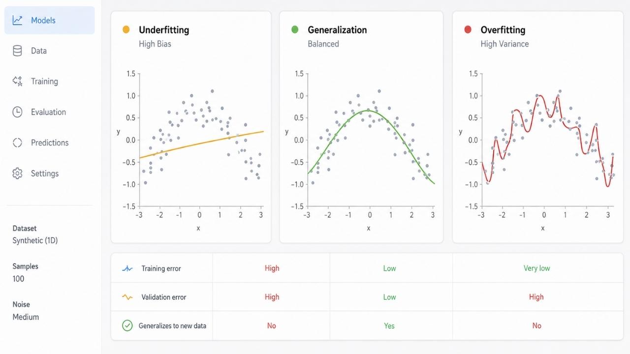
Overfitting happens when a model adapts too tightly to its training environment. The model captures short-term quirks in the training batch rather than signals that hold up across broader populations.
Take a basic decision tree built for spam filtering. Without depth limits, it might learn that emails containing “invoice” sent specifically on Tuesday afternoons are spam. That rule works on yesterday’s logs, but fails on almost everything else because it won’t generalize to tomorrow’s inbox.
High Bias (Underfitting)          Balanced Generalization           High Variance (Overfitting)

      Y |  x   x   /                 Y |  x   x  /                    Y |  x--x   /
        |    x    /                    |    x   /--x                    |   \  \ / x
        |  x   x /                     |  x   x/   x                    |  x \--X---x
        +----------->                  +----------->                    +----------->
             X                                X                                X
 Model is too simple.          Model captures trend.       Model memorizes noise.
Overfitting vs. Underfitting
Diagnosing the problem requires checking where the model sits on the bias-variance curve:
- Underfitting (High Bias): The architecture lacks the capacity to capture basic trends in the data. For example, forcing a linear model onto non-linear data leaves significant error across all splits.
- Overfitting (High Variance): The model is overly sensitive to small fluctuations. Training loss drops near zero, but validation error spikes.
- Generalization: The ideal state where performance remains consistent from validation to live deployment.
The Primary Causes of Overfitting
Overfitting in machine learning rarely stems from a single line of code. It usually reflects a disconnect between your dataset size, model capacity, and training duration.
Excessive Capacity
Architectures with millions of parameters easily memorize raw data if left unconstrained. With excess capacity, optimization algorithms fit individual data points instead of learning general trends.
Sparse or Imbalanced Datasets
In small datasets, random fluctuations look statistically significant to a high-capacity model. If most dog photos in a small dataset feature grassy backgrounds, a CNN might classify green pixels instead of canine features.
Data Leakage
Data leakage occurs when holdout information influences the feature engineering or preprocessing stage. Typical examples include:
- Computing normalization statistics (like mean or variance) across the entire dataset before splitting.
- Shuffling time-series samples randomly, which exposes historical splits to future state data.
Training Too Long
As gradient descent progresses, training loss will naturally continue to drop. Past a certain threshold, additional training runs only fit the residuals of that specific batch.
How to Detect Overfitting Early
Evaluating performance strictly on training data is misleading. The true indicator of overfitting in machine learning is a widening gap between training and validation loss.
 Error
   ^
   |        Validation Error (Starts rising -> Overfitting)
   |          \        /
   |           \------/
   |            \
   |             \----------- Training Error (Keeps dropping)
   +--------------------------------------------->
                   Training Time / Epochs
Comparing metrics across splits helps identify the model state:
| Metric State | Training Performance | Validation / Test Performance | Diagnostic |
| State A | Low (e.g., 65%) | Low (e.g., 62%) | Underfitting: Model lacks capacity or features. |
| State B | High (e.g., 99%) | Low (e.g., 71%) | Overfitting: High variance; memorizing training set. |
| State C | High (e.g., 92%) | High (e.g., 90%) | Balanced: Strong generalization across environments. |
Practical Techniques to Fix Overfitting

Fixing high variance requires intervention at the data layer, the architecture level, or the training loop.
1. K-Fold Cross-Validation
A fixed 80/20 split often masks variance, particularly on smaller datasets. K-Fold validation evaluates stability across multiple subsets:
- Divide the training set into $K$ equal folds.
- Train on $K-1$ folds and evaluate on the holdout fold.
- Rotate the holdout fold across $K$ runs and average the results.
If performance metrics swing wildly between folds, your model is overly sensitive to training variations.
2. Regularization ($L_1$ and $L_2$)
Regularization adds a penalty term to the loss function to constrain weight growth and simplify model behavior.
-
$L_1$ Regularization (Lasso): This zeros out coefficients for uninformative features, simplifying the model:
-
$L_2$ Regularization (Ridge): This shrinks weights uniformly, preventing individual variables from dominating the output:
The scalar $\lambda$ controls how heavily large weights are penalized.
3. Early Stopping
For iterative models, early stopping halts training once validation metrics stop improving. Define an evaluation window—such as 10 epochs without validation progress—before triggering a stop and restoring the best weights.
4. Dropout
In deep networks, adjacent layers often become overly dependent on specific joint weights. Dropout mitigates this by zeroing out a random subset of activations (usually 20% to 50%) during each training step. This encourages redundant feature pathways rather than brittle, single-node dependencies.
     Standard Layer                    Layer with Dropout (p = 0.5)
    (O)---(O)---(O)                     (O)   [X]   (O)
     \   /   \   /                        \       \   /
      (O)---(O)---(O)                     [X]---(O)   [X]
     /   /   \   /                        /       /   /
    (O)---(O)---(O)                     (O)   [X]   (O)
5. Data Augmentation
When collecting more data isn’t an option, synthetic expansion adds variance:
- Vision: Apply random cropping, subtle rotations, and horizontal flips.
- Text: Use synonym substitution or back-translation.
- Tabular Data: Introduce Gaussian noise or generate synthetic minority samples using SMOTE.
6. Constraining Model Architecture
Directly limiting model capacity is often the most straightforward fix:
- Trees: Set upper bounds on
max_depthand require higher values formin_samples_leaf. - Neural Networks: Reduce layer counts or narrow channel widths.
- Tabular Features: Drop low-variance inputs or compress high-dimensional spaces using PCA.
Common Implementation Mistakes
Over-Correcting Into Underfitting
Stacking strict tree depth limits, high dropout rates, and strong regularization all at once usually induces high bias. If both training and validation errors remain unacceptably high, ease off on the penalties.
Leakage During Preprocessing
If you fit your scalers or imputers on the full dataset before splitting, information from the test set leaks into training, yielding overly optimistic metrics. Always keep preprocessing logic inside cross-validation loops or pipeline transformers.
Hyperparameter Tuning on the Test Set
Repeatedly running experiments to maximize scores on a single validation split causes subtle validation-set memorization. Always keep a dedicated holdout test set untouched until final evaluation.
Practical Pipeline Checklist
Follow this workflow to keep overfitting in machine learning under control:
- Start Simple: Fit a basic linear model or shallow tree to establish a baseline.
- Isolate Holdout Data Immediately: Separate test data before running feature engineering or scaling.
- Establish Cross-Validation: Track performance stability across data splits rather than relying on a single test score.
- Enable Guardrails Early: Apply baseline regularization rules from day one.
- Monitor Loss Curves: Graph training loss against validation loss continuously to spot divergence points early.
Final Thoughts
Preventing overfitting in machine learning isn’t about aiming for zero training error—it’s a standard trade-off when working with high-capacity models. Handling it comes down to good habits: strict data boundaries, early cross-validation, and proportional regularization. Keeping model capacity in check is what makes the difference between a high benchmark score and a working production system.