

How to choose an enterprise LLM API starts with the work you need it to complete: the quality you will accept, the time your users can wait, the data boundaries you must preserve, and the cost of a successful outcome. A low token price or a large context window answers only part of that decision. You need to compare the model, delivery platform, region, service tier and contract together.
For a practical shortlist, start with two or three eligible deployments. Test the same representative tasks, measure response times under expected load, calculate the full bill, and require a workable recovery plan. Choose the option that meets your quality and operational requirements at a sustainable cost; keep a second route only when you can maintain and test it.
How This Guide Was Checked
This guide draws on official OpenAI, Anthropic, Microsoft, AWS and Google Cloud documentation checked on November 15, 2026, alongside Stanford’s evaluation framework and NIST’s risk-management guidance. Its original contribution is an assistant-executed, reproducible cost calculation using published rates and explicitly hypothetical workloads; no provider API calls, paid-account trials or live latency benchmarks were performed.
You can inspect the assumptions and results in the cost tables below. The benchmark procedure is a proposed pilot for your team, not a report of tests already completed. Provider examples illustrate procurement choices rather than a measured ranking.
How to Choose an Enterprise LLM API: Start With These Gates
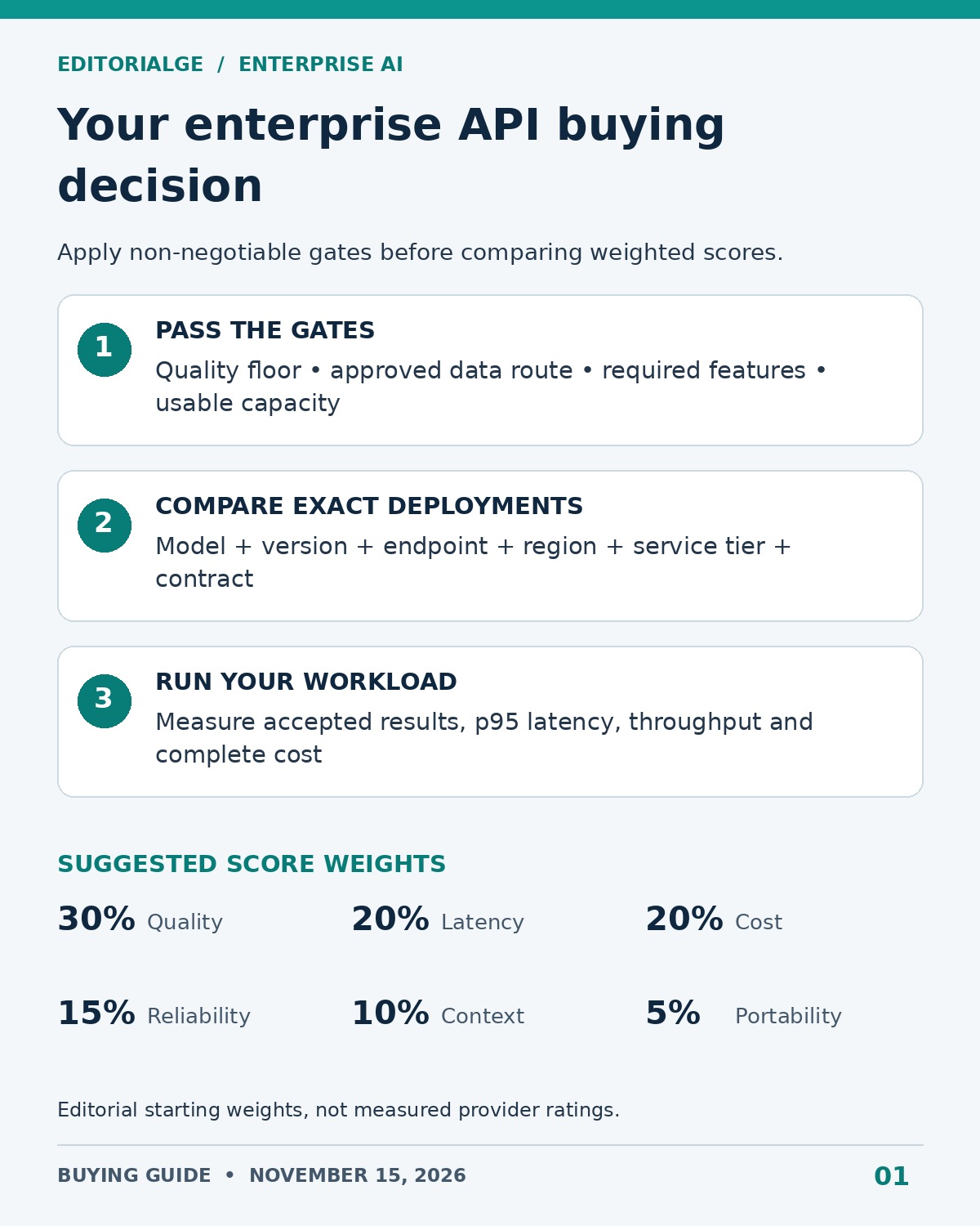
Before you score a provider, eliminate deployments that cannot satisfy your essential requirements. A high overall score should never compensate for sending restricted data to an unapproved location or failing a critical extraction task.
| Decision gate | What you need before proceeding | What should stop the purchase |
|---|---|---|
| Task quality | A versioned test set and agreed acceptance criteria | Unacceptable factual errors, missing fields or unsafe tool actions |
| Data and access | Approved processing route, retention terms and access controls | An unresolved data-handling requirement |
| Deployment eligibility | The exact model and necessary features in your intended region and tier | A capability available only on a different endpoint |
| Capacity | Usable quota or reserved capacity at your expected peak | A production launch dependent on an unapproved quota increase |
| Commercial terms | Budget limits, support ownership, incident terms and an exit plan | A commitment you cannot justify at conservative utilization |
Write a one-page workload brief before requesting quotes. Include monthly task count, peak requests per second, typical and unusually large inputs, expected output length, languages, tool calls and permitted regions. Separate customer-facing chat from overnight processing: their acceptable delays are different.
For governance, you can use the voluntary NIST AI Risk Management Framework to organize risk ownership and evaluation. It does not certify a particular provider or replace your review of the actual deployment.
Compare the Buying Route Before the Model Name
Your provider choice has two layers: which model generates the answer, and which service delivers it. Treat each proposed configuration as a separate candidate. Record its exact model identifier, endpoint, region, version policy and billing owner in the comparison sheet.
| Route to shortlist | When it deserves consideration | What changes the decision |
|---|---|---|
| OpenAI direct API | You want to evaluate OpenAI models through the provider’s own API and service tiers | Compare the selected context band, processing tier, caching and regional charges |
| Anthropic direct API | You want to evaluate Claude with its documented model and caching options | Price cache writes, reads and output separately; partner-operated routes have separate billing terms |
| Microsoft Foundry / Azure OpenAI | You want to evaluate an Azure deployment alongside your existing cloud operations | Standard quota is not a throughput promise; provisioned capacity depends on workload shape |
| Amazon Bedrock | You want an AWS purchasing and operational route for supported models | Check model availability and the relevant on-demand or provisioned configuration; reserved capacity can carry commitments |
| Google Cloud’s Gemini service | You want to evaluate Gemini through Google Cloud and its capacity options | Match the exact model and endpoint to pricing, availability coverage and any latency commitment |
These are starting points for procurement, not claims that one platform is universally better. Existing cloud approval can make a route worth investigating, but you still need to establish whether its model version, tools and operating terms match the application you plan to ship.
API compatibility also needs a practical check. Successful text generation does not establish equivalent behavior for structured output, tool calls, streaming events or error handling. Keep a small set of integration tests that exercise the features your application actually uses.
Measure Latency Across the Entire User Journey
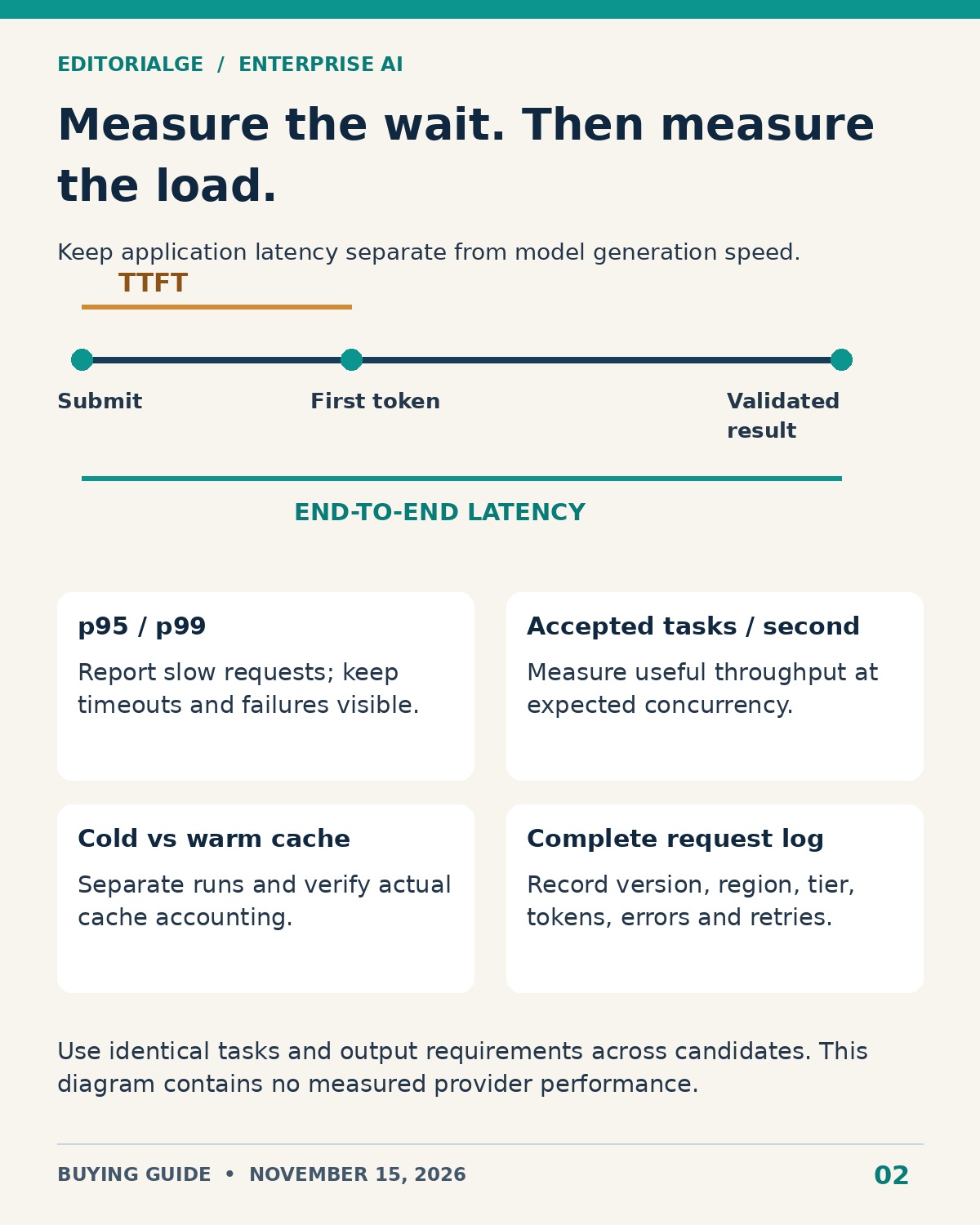
Latency is the time a request takes. Throughput is the work a system completes over time. You need both: a deployment can answer one request quickly and still struggle when many users arrive together.
| Metric | What you measure | Why it matters |
|---|---|---|
| Time to first token (TTFT) | Request submission to the first generated content token | How quickly a streamed response starts; record first user-visible text separately if filtering delays display |
| End-to-end latency | User action to a complete, validated result | Includes retrieval, tool calls, generation, validation and retries |
| Generation speed | Generated tokens divided by the explicitly defined generation interval | Explains the wait after generation begins; it is not total application speed |
| Successful throughput | Accepted results completed per second or minute | Shows useful capacity under load, including the effect of failures |
| Tail latency | p95 and, with enough samples, p99 response time | Exposes slow requests hidden by averages |
A p95 of four seconds means 95% of measured requests completed within four seconds in that sample. It says nothing about the severity of the remaining delays unless you inspect them. Report failed requests and timeouts separately; quietly removing them makes a struggling service look faster.
Microsoft’s performance documentation explicitly distinguishes deployment quota from achieved throughput. Its provisioned throughput also varies with input length, output length, call rate and cache behavior. That makes a quota screenshot inadequate evidence of production capacity.
OpenAI’s latency guidance describes streaming and stable prompt prefixes as useful techniques. Streaming can let your user read earlier, while prefix reuse may reduce repeated input processing. Neither removes the time required for dependent tools, checks or later generation. Measure the complete workflow before promising a faster experience.
How to Run Useful LLM Throughput Benchmarks
Use the same task corpus across candidates and each provider’s own token accounting. The same text can produce different token counts, so forcing an identical token count may change the underlying task. Keep output requirements, reasoning settings where comparable, tool permissions and acceptance criteria explicit.
- Freeze a representative dataset with expected answers or a grading rubric. Include ordinary work, long inputs, ambiguous instructions and cases where the correct response is to abstain.
- Record model/version, region, endpoint, service tier, SDK version, retry settings and test-client location. Preserve the original configuration beside your results.
- Test cold and warm cache conditions separately. Confirm cache usage from returned accounting instead of assuming repeated prompts produced hits.
- Increase concurrency in steps until you reach expected peak load and a modest safety margin. For example, 1, 5, 10 and 25 concurrent requests can be a pilot ladder, not a universal capacity target.
- Run repeated samples in several time windows. A few hundred requests per configuration can reveal obvious problems, but a stable p99 estimate generally needs substantially more observations.
- Log initial failures, retry attempts, final outcomes, input/output usage, TTFT and completion time. Distinguish network failures, rate limits, server errors and incorrect answers.
- Review quality blind to provider where practical. Compare only candidates that clear your quality floor, then repeat the final configuration with retrieval and downstream tools enabled.
Stanford’s HELM framework offers transparent, reproducible evaluation across scenarios and metrics. You can use public evaluations to narrow a shortlist, but they cannot establish the latency, task success or regional capacity of your own application.
Define an initial target in application terms: for example, “95% of accepted support drafts must be ready within six seconds at ten concurrent requests.” This is an illustrative requirement you can replace, not a provider benchmark. Retain enough detail to explain whether a failure came from the model or another part of your system.
Buy Usable Context, Not Just a Large Advertised Window
A context window limits how much information a model can work with in a request or conversation. It is separate from maximum output length. Provider definitions and accounting vary, so check both limits and leave room for instructions, tool definitions, conversation history, retrieved material and any model-specific reasoning requirements.
For a hypothetical deployment with a 128,000-token combined budget, you might allocate 12,000 to instructions and tools, 90,000 to documents, 10,000 to history and 12,000 to output, leaving 4,000 tokens of headroom. This arithmetic is a planning example, not a specification for the providers below.
| Documented example, checked November 15, 2026 | Advertised context | Maximum output | Procurement implication |
|---|---|---|---|
| GPT-6.1 Sol, OpenAI direct | 1.05 million tokens | 128K tokens | Its API page distinguishes standard prices for context under 272K from longer-context pricing |
| Claude Sonnet 5.5, Anthropic direct | 1 million tokens | 128K tokens | A long window still requires validation of the exact documents and instructions you send |
| Gemini 2.5 Pro, Google Cloud documentation | 1,048,576 tokens | 65,536 tokens | The published price table has different rates above 200K input tokens |
These are selected documented examples, not a claim that all three are the newest models or equally suitable. A large window does not establish accurate synthesis across every passage. Put relevant facts at different positions, include conflicting and outdated documents, and require source-grounded answers. Test whether your application catches a plausible but unsupported response.
Compare full-context processing with retrieval on the same questions. Retrieval can reduce input volume, but missed passages may harm answers; a large prompt can retain more material, but it increases the amount to process. Your choice should follow answer quality and end-to-end cost. Editorialge’s guide to AI token optimization tools explains the different roles of context selection, compression and caching.
Token Pricing Tiers: Build a Complete Cost Breakdown
Start with billable usage categories. Avoid multiplying a provider’s cheapest input price by all tokens: output, cache writes, cache reads and other services may have different rates.
Token cost = (uncached input × input rate + cache-write tokens × write rate + cached input × read rate + billable output × output rate) ÷ 1,000,000
In this formula the three input categories are mutually exclusive. Normalize provider usage fields before applying it so that you do not bill a cached token twice. Add storage or retention charges, embeddings, retrieval, tool execution, gateways, monitoring, support, reserved capacity and any applicable taxes separately. Include reasoning tokens according to the selected model’s billing definition.
A Dated Price Snapshot, With Matching Assumptions
The following published USD rates were checked on November 15, 2026. The monthly scenario assumes 100,000 requests with 4,000 uncached input tokens and 800 billable output tokens each: 400 million input and 80 million output tokens. It excludes tools, caching, retries, discounts, taxes and infrastructure. It is a calculation, not an observed invoice or quality comparison.
| Model and purchase route | Input / 1M tokens | Output / 1M tokens | Calculated token cost |
|---|---|---|---|
| GPT-6.1 Sol, OpenAI direct, Standard, short context | $2.00 | $10.00 | $1,600 |
| Claude Sonnet 5.5, Anthropic direct, base rates | $2.00 | $10.00 | $1,600 |
| Gemini 2.5 Pro, Google Cloud, standard requests at or below 200K input | $1.25 | $10.00 | $1,300 |
The Google Cloud price table lists $2.50 input and $15 output per million tokens for Gemini 2.5 Pro requests above 200K input. A threshold can therefore change more than the price of the extra tokens. Check the rule for the whole request before extrapolating from a short-context quote. The table’s equal token volumes also do not imply equal text length across tokenizers.
Original Calculation: What Caching Changes
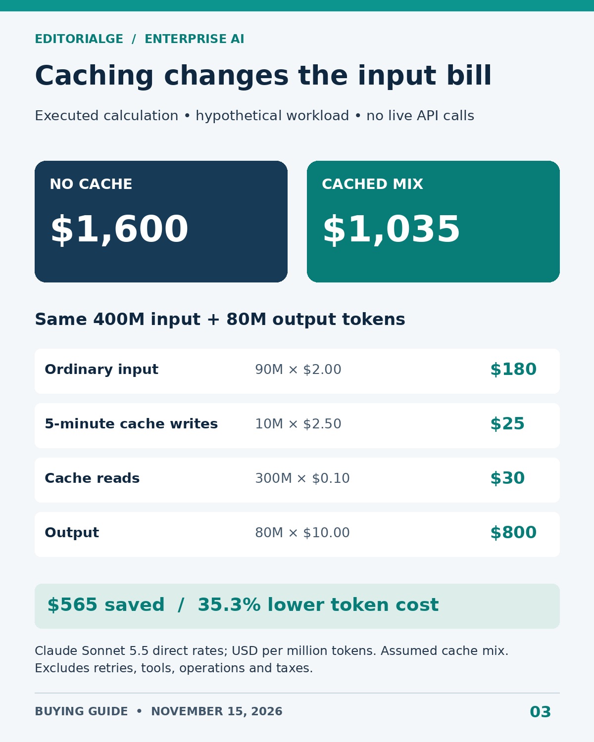
The locally executed calculation uses Claude Sonnet 5.5’s published direct rates: $2 per million ordinary input tokens, $2.50 for five-minute cache writes, $0.10 for cache reads and $10 for output. For the same hypothetical 400-million-token input workload, assume 90 million ordinary input tokens, 10 million write tokens and 300 million read tokens; keep output at 80 million.
| Billable component | Without caching | Illustrative cached workload |
|---|---|---|
| Ordinary input | 400M × $2 = $800 | 90M × $2 = $180 |
| Five-minute cache writes | $0 | 10M × $2.50 = $25 |
| Cache reads | $0 | 300M × $0.10 = $30 |
| Output | 80M × $10 = $800 | 80M × $10 = $800 |
| Total | $1,600 | $1,035 |
The calculated reduction is $565, or 35.3%. Although cache reads cover 75% of input tokens, they do not reduce the unchanged $800 output cost. The assumed cache mix is not a measured hit rate; your prefix reuse, expiration and refresh behavior determine the real mix.
Now add a hypothetical 20% of extra billable work with the same usage mix: $1,035 becomes $1,242. Add $200 of operational costs and the total reaches $1,442. If 95,000 tasks are accepted, your cost per accepted task is about $0.0152. This scenario does not assume every failed HTTP request is billed; the extra work represents billable retries, repeated generations or fallback calls.
Use this outcome-based denominator when comparing models with different success rates. You should also assign spend to the responsible product, customer or department; the AI showback and chargeback guide covers that operational step.
Reproduce the Cost Calculation
You can run the following Python calculation without an API key or a paid account. Each input quantity is in millions of tokens, so multiplying it by the corresponding per-million-token rate gives the cost in USD. The input categories are disjoint: ordinary input, cache writes and cache reads.
from decimal import Decimal as D

uncached = D("400") * D("2") + D("80") * D("10")
cached = (
    D("90") * D("2")
    + D("10") * D("2.50")
    + D("300") * D("0.10")
    + D("80") * D("10")
)
saving = (uncached - cached) / uncached * D("100")

print(f"Without caching:
Choose a Pricing Tier That Matches Demand
#123;uncached:.2f}”) print(f”With assumed cache mix:
Choose a Pricing Tier That Matches Demand
#123;cached:.2f}”) print(f”Reduction: {saving:.4f}%”)
The executed result is $1,600.00 without caching, $1,035.00 with the assumed cache mix, and a 35.3125% reduction. This verifies the arithmetic under the stated assumptions; it does not verify that a production application will achieve that cache mix.
What This Calculation Means for Your Shortlist
The practical recommendation is to control output length as carefully as repeated input. In the cached scenario, output accounts for $800 of the $1,035 total. If billable output doubles from 80 million to 160 million tokens while the same input mix is retained, the calculated total rises to $1,835. That sensitivity check is a reason to compare concise, accepted answers rather than rewarding a provider simply for generating more text.
Keep quality as a hard requirement: shortening a response is useful only when it still completes the task. Treat this recommendation as an interpretation of the disclosed cost model, and validate its relevance with your own usage before making a commitment.
Choose a Pricing Tier That Matches Demand
On-demand pricing is useful when your workload is uncertain or bursty. Batch processing deserves a separate comparison when you can tolerate asynchronous completion. Premium processing may justify its cost for interactive workflows, but you should measure its improvement on your own requests.
Reserved or provisioned throughput needs a utilization forecast. AWS documents hourly billing for provisioned model units, with available commitment choices depending on configuration. A lower unit cost at high utilization can become expensive when traffic is intermittent. Compare the committed monthly total plus overflow against your on-demand forecast; do not divide a reservation by its theoretical maximum capacity and call that your effective price.
SLA Reliability: Read What the Promise Actually Covers
An SLA defines a contractual service commitment and the remedy when its conditions are met. Your application’s service-level objective is the experience you intend to deliver. They may measure different events, and neither automatically proves answer accuracy.
For a simple 30-day time-based illustration, 99.5% availability corresponds to 216 minutes outside the target, 99.9% to 43.2 minutes and 99.99% to 4.32 minutes. Actual SLA calculations can use request errors, time intervals and exclusions instead of this simple clock calculation.
Amazon Bedrock’s published terms calculate availability using defined request errors and five-minute intervals, with service credits and a claims process. Google Cloud’s Gemini Online Inference SLA lists a 99.5% monthly uptime objective, with a lower objective for designated shorter-availability models. Its separate provisioned-throughput latency commitment is limited to specified models, a covered endpoint and qualifying conditions. These examples show why “enterprise SLA” is too vague for a buying decision.
Ask for the current contract schedule for your exact deployment. Confirm coverage for the model, region and tier; whether latency means TTFT, token generation or another measure; which errors count; exclusions; credit caps; evidence requirements; and the deadline for submitting a claim. A support response target is also different from a restoration target.
Design recovery separately. Use bounded retries with backoff, prevent retry storms, set a request deadline and provide a useful degraded response where possible. A second provider helps only if its capacity, quality and data route are already approved. Test failover with controlled errors and keep duplicate side effects out of payment, account or other action-taking workflows.
Use a Weighted Decision Matrix After the Gates
The following weights are an editorial starting point for an interactive enterprise application. Adjust them before you see provider results. Score each criterion from one to five using written thresholds, and attach evidence to every score.
| Criterion | Suggested weight | Evidence to score |
|---|---|---|
| Task quality | 30% | Accepted answers, field accuracy, groundedness and critical failures |
| Latency under load | 20% | p95 end-to-end time and successful throughput at expected concurrency |
| Cost per accepted task | 20% | Complete usage and operating costs divided by accepted outcomes |
| Reliability and recovery | 15% | Observed errors, recovery exercises and applicable service terms |
| Usable context | 10% | Performance on realistic long inputs, limits and price thresholds |
| Portability and operations | 5% | Integration effort, version control, monitoring and exit cost |
Weighted score out of 100 = sum of (criterion weight × rating ÷ 5)
For illustration, ratings of 4, 5, 3, 3, 4 and 4 produce 77/100 with these weights. That is a fictional worked example, not a score for any named provider. Repeat the decision with cost or latency weighted more heavily: if a small change reverses the winner, record the trade-off instead of presenting a decisive ranking.
Keep governance as a pass/fail gate. For overnight document processing, you might move weight from interactive latency to cost and quality. For a time-sensitive customer service workflow, you may emphasize tail latency and recovery. The matrix should reflect your business, not a universal league table.
Turn the Shortlist Into a Purchase Decision
Ask each finalist to respond to the same workload brief. Request the exact model and endpoint, production quota, price schedule, context thresholds, commitment terms, support escalation path and deprecation notice policy. Clarify how prompts, outputs, logs and cached data are handled across both the model service and your own observability systems.
Your pilot should end with a short recommendation: which deployment passed, which requirements remain unmet, what the expected monthly range is, and who owns rollout and recovery. Include the conditions that would trigger reconsideration, such as a material price change, a retired model version, reduced acceptance rate or persistent tail-latency breach.
Before committing, keep an exportable evaluation dataset, configuration record and usage report. Preserve a small adapter boundary in your application, but budget for retesting when you change providers. Similar APIs make migration easier; they do not remove differences in behavior.
Frequently Asked Questions
Which enterprise LLM API provider is best?
The strongest choice is the eligible deployment that meets your quality, data, capacity and response-time requirements at the lowest sustainable total cost. You cannot identify it from a model leaderboard or token price alone.
What matters more: latency or throughput?
You need latency for individual user waits and throughput for peak demand. Compare p95 completion time and accepted results per second at the same workload and concurrency, rather than choosing one metric in isolation.
Does a million-token context window replace retrieval?
It can make some full-document workflows practical, but it does not establish retrieval accuracy or answer quality. Compare both approaches on your documents, including conflicting facts and evidence located deep in the input.
Are cached tokens free?
No. A provider may price reads, writes and retention differently. Calculate savings from actual usage fields, and include output and other services rather than applying a cache discount to the entire bill.
Does an SLA guarantee fast responses?
Only a relevant performance commitment can support that expectation, and it remains subject to its definitions and exclusions. An availability SLA alone does not guarantee your application’s response time or the correctness of an answer.
What original testing supports this guide?
The cost arithmetic was executed locally from documented prices and disclosed hypothetical inputs. You can reproduce its totals from the tables. No live provider performance or reliability measurement is presented; those require the workload pilot described above.
Your Final Decision
How to choose an enterprise LLM API becomes a manageable procurement exercise when you define the workload first. Apply the hard gates, compare exact deployments, measure useful performance, and calculate cost per accepted task. Then choose the provider whose operating terms and recovery plan you can support in production, with a documented reason to revisit the decision as your workload changes.