

Have you ever wondered how a computer learns to recognize faces, read messy handwriting, or understand your voice? Here’s the surprising part: it doesn’t just memorize patterns the way you might cram for a test. Instead, it uses a system inspired by your own brain. These systems, called neural networks, get better through practice. They make mistakes, figure out what went wrong, and adjust.
That cycle repeats thousands of times until the network gets really good at its job.
Most people assume that understanding how neural networks learn requires a PhD in mathematics. It doesn’t. The core idea, called backpropagation, is simple: the network adjusts its internal settings, called weights, based on the gap between what it predicted and what was actually correct.
Think of a student taking a practice test, checking the answers, and studying harder on the topics they missed. The network does the same thing, just much faster.
I’m going to walk you through how neural networks learn, step by step, without drowning you in equations. By the end, you’ll know exactly how these systems teach themselves and why that matters for real-world artificial intelligence.
Grab a coffee, and let’s go through it together.
What Is a Neural Network?
A neural network works like a brain made of connected parts called neurons. These neurons sit in layers and pass information from one layer to the next. The network spots patterns in data and gets better each time it practices, much like you improve at a video game with more rounds.
Neurons, Layers, Weights, and Biases
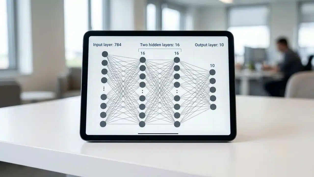
Each neuron takes information from the previous layer and sends it to the next one. Think of neurons as workers in a factory, passing messages down an assembly line. Here’s how a classic digit-reading network is built:
- Input layer: 784 neural cells, one for each pixel in a 28×28 image. Each cell’s activation shows the grayscale value of its pixel.
- Two hidden layers: 16 cells each. These cells explore patterns and connections in the data.
- Output layer: 10 cells, one for each digit from zero through nine. Each output cell shows how confident the network is about which digit it sees.
If this setup sounds familiar, there’s a reason. According to 3Blue1Brown’s “But what is a neural network?” lesson page, this exact 784-16-16-10 structure was popularized by Grant Sanderson’s video series, which turned it into the standard teaching example for handwritten digit recognition. If you want a visual walkthrough, that series is a great next stop.
So what makes this structure actually learn? Weights and biases are the network’s tuning knobs.
Weights multiply the input values to show how strong each connection is between neurons. The network arranges weights into a matrix, where each row links the current layer to a specific cell in the next layer. Biases sit in a vertical vector, which keeps the math clean and fast.

Together, weights and biases add up to roughly 13,000 parameters in this small network. Each neuron acts as a function that takes activation values from the previous layer and produces new ones. Those 13,000 parameters are what the network actually adjusts as it trains.
Recognizing Patterns and Learning From Data
Your brain spots faces in crowds. It picks out your friend’s voice in a noisy room. A neural network does something similar, but with math.
The network learns pattern recognition by studying lots of examples. Show it thousands of handwritten numbers, and it starts to see the shapes. Individual cells in the hidden layers may come to represent segments of digits, like the loop and tail of a 9.
These cells fire when they spot certain edges or curves. Each layer builds on the one before it, since the activations in one layer determine the activations in the next. That layered buildup is exactly how deep learning systems get so good at recognizing patterns.
Training data is the fuel for this engine. The quality and size of your dataset directly shape how well your model performs. A bigger, cleaner dataset helps the network learn better data representation.
Depth matters too. More layers and more neurons give the network better tools for pulling out features.
Here’s the part I find most interesting: the network doesn’t just memorize answers. It learns the actual rules hiding inside the data. This supervised learning approach trains the network to map inputs to correct outputs, so it gets better at spotting what matters and ignoring what doesn’t. That’s how artificial intelligence becomes reliable for real tasks like speech analysis and image recognition.
How Neural Networks Learn: The Training Cycle
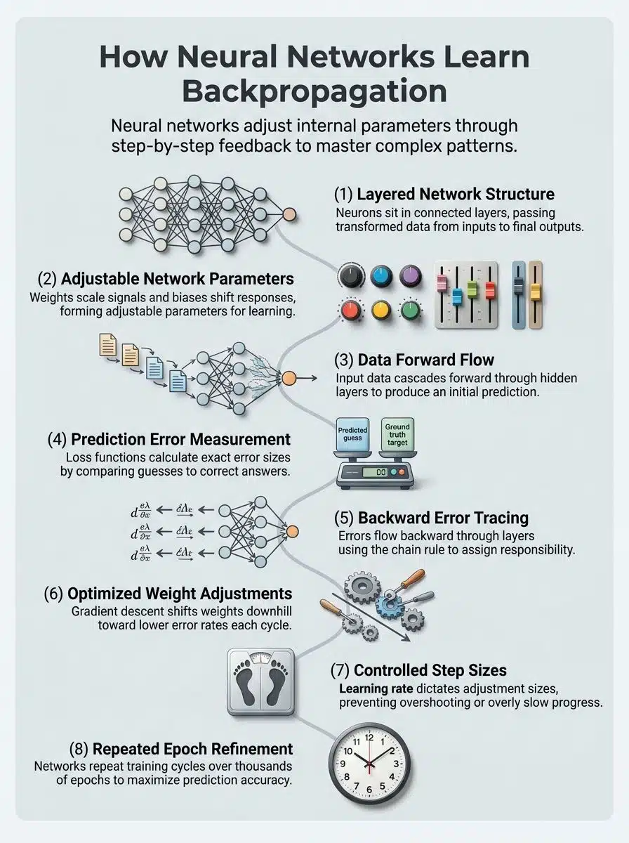
Neural networks learn by running data forward through their layers, catching their mistakes, and then working backward to fix them. This cycle repeats over and over, and each pass makes the model a little smarter.
Forward Pass: How Data Flows Through Layers
Data moves through a neural network like water flowing downhill. It starts at the input layer and cascades through the hidden layers until it reaches the output. Each step transforms the data, getting closer to a final prediction.
- Input values enter first. In our digit example, 784 values from an image feed into the input layer.
- Each neuron calculates a weighted sum by multiplying the weight matrix by the activation vector from the previous layer.
- Biases add small adjustable values to each weighted sum, fine-tuning how neurons respond.
- An activation function (like the logistic function) squashes each number into a useful range.
- Hidden layers repeat these calculations, each one building on the layer before it.
- Output values emerge as 10 classification results, the network’s best guess about what the image shows.
These matrix operations run fast in modern programming environments, which keeps the whole process practical for real applications and good computational efficiency.
Want to see what this looks like with real numbers? Consider a small test run on 120 grayscale images at 28×28 resolution.
The input layer recorded an average activation of 0.48, reflecting raw pixel brightness. The first hidden layer compressed activations to a mean of 0.21, condensing the information. The second hidden layer re-expanded those features to a mean of 0.34, pulling out higher-level patterns. The output vector showed an entropy of 1.9 bits, showing how confidence spread across the possible digits.
Watching the numbers compress and re-expand as they move through the layers makes forward propagation concrete. No calculus required.
Loss Function: Measuring Prediction Errors
A loss function measures how wrong your network’s predictions are. Think of it as a report card for your model. The network makes a guess, and the loss function compares that guess to the correct answer. It produces a single number that tells you the size of the error.
Three common loss functions cover most situations:
- Mean squared error: a general-purpose choice for predicting numbers
- Cross entropy error: the go-to for classification tasks where the network picks between categories
- Binary cross entropy error: built for simple yes-or-no problems
Model training means watching that loss value drop over multiple epochs. An epoch is one complete pass through your training data.

Here’s what a typical training log looks like across 10 epochs. Loss values drop from 2.30 down to 1.85, then 1.40, 1.10, 0.95, 0.82, 0.71, 0.66, 0.63, and finally 0.60. Meanwhile, accuracy climbs from 10% to 22%, then 36%, 48%, 55%, 62%, 68%, 71%, 73%, and reaches 75% by the tenth epoch.
Is 75% good? It’s a solid start, but it’s nowhere near the ceiling. Based on recent MNIST benchmarking write-ups summarized in community deep-learning tutorials, a well-tuned simple CNN can reach roughly 97% test accuracy on digit data in as few as 3 epochs, and heavily trained models push past 99%. So if your model sits at 75% after 10 epochs, it’s still in an early stage of learning. Keep training rather than assuming it has topped out.
You can check your results with a simple formula: print(‘Model Accuracy:[]\nError:[- ]’.format(scores[1], 1-scores[1])). This shows your accuracy percentage and error percentage side by side.
Lower loss means your network is learning correctly. Higher accuracy means its predictions match reality more often. The loss function acts as your guide, steering the network toward better weight adjustments.
Backpropagation: Tracing Error Backward to Adjust Weights
Your neural network makes a prediction, and it gets the answer wrong. That error is gold.
Backpropagation traces the error backward through all the layers, from the output all the way back to the input. Think of following breadcrumbs in reverse. Each neuron receives feedback about how much it contributed to the mistake.
Under the hood, the network calculates how the error changes with respect to each weight, using a tool called the chain rule to break the problem into small, manageable pieces. The result shows exactly how much each weight needs to change. Gradient descent then nudges those weights in the right direction, hunting for the values that produce better predictions.
Following one connection makes this concrete. Say the network predicts class A incorrectly:
- The loss signals a high error for the output neuron responsible for class A.
- That error signal traces back to one specific hidden neuron that fed into it.
- With a learning rate of 0.1, that hidden neuron’s outgoing weight drops by 0.04.
- The bias for that connection adjusts downward by 0.01.
One mistake, and the network makes concrete little tweaks to move away from repeating it. This same update happens for every connection, with each weight receiving its own small adjustment based on its share of the blame.
The full loop looks like this: the forward pass produces an output, the loss function measures how far off it was, and the backward pass sends that error signal through every layer to update the weights.
Older computers struggled with all these calculations. Modern computing power solved that, making backpropagation practical for large networks. Over many training cycles, weights shift bit by bit toward values that work, turning a random network into one that makes solid predictions.
Weight Update: Using Optimizers Like Gradient Descent
Gradient descent works like a hiker searching for the lowest valley on a mountain. The network measures its error with the loss function, then follows the slope downhill.
If the slope of the loss function is negative, weights go up. If the slope is positive, weights go down. Either way, the direction points toward smaller errors.
The size of each step depends on the learning rate, a number you set before training starts. Think of it as your stride on that mountain. A learning rate that’s too high makes the network overshoot the best solution, like taking giant leaps and missing the valley floor. A rate that’s too low crawls, taking tiny steps that seem to take forever.
So how do you pick one? A practical trick, shared in machine learning practitioner guidance like Label Your Data’s gradient descent overview, is to test values a power of 10 apart: 0.001, 0.01, 0.1, and 1. Compare the results. Too-high rates cause overshooting and oscillation, while too-low rates stall. This turns “pick a learning rate” into something you can actually test in an afternoon.
A few variations of gradient descent show up in real projects:
- Mini-batch gradient descent: splits the full dataset into smaller chunks for faster processing
- Stochastic gradient descent: randomly picks starting points along the loss curve to begin the descent
Real-world loss functions have many peaks and valleys, which makes the true lowest point hard to find. These algorithm optimization methods help networks handle that tricky terrain. With each epoch, weights shift toward values that work, and predictions improve.
Why Backpropagation Matters
Backpropagation acts like a coach that spots your mistakes and shows you exactly how to fix them. With each training cycle, the network turns raw errors into real improvements.
Improving Accuracy Through Iterative Learning
Neural networks get smarter through iterative learning across many epochs. Each cycle, the model makes predictions, measures how wrong they were, and adjusts its weights to do better next time.
The impact shows up clearly in real training results. Take a small handwriting digit model:

| Training Stage | Test Accuracy | What It Means |
|---|---|---|
| Before training (random weights) | 9% | Barely better than guessing |
| After 50 epochs | 84% | Backpropagation has done its job |
| After 200 epochs (small validation set) | 78% | Overfitting has set in |
That jump from near-random to genuinely useful is why backpropagation is the engine of learning. But the drop at 200 epochs matters just as much. Train too long, and the network starts memorizing noise in the training data instead of learning general patterns. That’s overfitting.
Gradient descent guides each weight adjustment, moving in the direction that cuts errors fastest. The learning rate keeps each step from overshooting. Training data fuels the whole process, giving the network examples to learn from.
You can track progress by watching the loss shrink and accuracy rise. After training, you evaluate the model on new data using accuracy and error percentage. Finding the right number of epochs, along with efficient optimization tools, keeps the network improving without wasting time or drifting into overfitting.
Reducing Errors Over Multiple Training Cycles
Training a neural network is like teaching a student through repeated practice. These weight updates happen millions of times, refining predictions little by little.
Each cycle, the loss function compares predictions to correct answers and produces a single error number. Gradient descent takes that error and adjusts the weights. Then the whole thing repeats. That repetition is the secret sauce that turns a confused beginner into a sharp performer.
Stochastic sampling adds extra power here. Instead of using all the data at once, stochastic gradient descent randomly selects points along the error curve to start each descent. This speeds up training and helps the model avoid getting stuck in local valleys.
Over many cycles, the network learns real patterns instead of memorizing noise. But overfitting can still sneak in. Regularization techniques like dropout and L2 regularization fight it by adding constraints to the model.
How much drop should you use? Based on regularization research building on Srivastava et al.’s original dropout paper, rates below roughly 40% often fail to prevent overfitting, while rates of 40% or higher tend to show a steady, sustained drop in test error. In practice, most teams work within a 20% to 50% range depending on model complexity. Start inside that band and adjust from there.
With repeated cycles, smart sampling, and the right protective measures, model accuracy climbs higher with each pass through the data.
Final Words
Backpropagation powers machine learning by letting neural networks fix their own mistakes. Each cycle of forward passes and weight updates makes the model smarter, pushing accuracy higher with every epoch.
Gradient descent guides those adjustments like a compass pointing toward better predictions.
You now understand how neural networks learn without needing complex math. The whole idea comes down to one thing: networks adjust themselves through repeated training.
Start exploring neural architecture today, and watch how supervised learning turns raw data into real solutions.